Single-Node Patterns
Though it is clear as to why you might want to break your distributed application into a collection of different containers running on different machines, it is perhaps somewhat less clear as to why you might also want to break up the components running on a single machine into different containers. To understand the motivation for these groups of containers, it is worth considering the goals behind containerization. In general, the goal of a container is to establish boundaries around specific resources (e.g., this application needs two cores and 8 GB of memory). Likewise, the boundary delineates team ownership (e.g., this team owns this image). Finally, the boundary is intended to provide separation of concerns (e.g., this image does this one thing).
All of these reasons provide motivation for splitting up an application on a single machine into a group of containers. Consider resource isolation first. Your application may be made up of two components: one is a user-facing application server and the other is a background configuration file loader. Clearly, end-user-facing request latency is the highest priority, so the user-facing application needs to have sufficient resources to ensure that it is highly responsive. On the other hand, the background configuration loader is mostly a best-effort service; if it is delayed slightly during times of high user-request volume, the system will be okay. Likewise, the background configuration loader should not impact the quality of service that end users receive. For all of these reasons, you want to separate the user-facing service and the background shard loader into different containers. This allows you to attach different resource requirements and priorities to the two different containers and, for example, ensure that the background loader opportunistically steals cycles from the user-facing service whenever it is lightly loaded and the cycles are free. Likewise, separate resource requirements for the two containers ensure that the background loader will be terminated before the user-facing service if there is a resource contention issue caused by a memory leak or other overcommitment of memory resources.
In addition to this resource isolation, there are other reasons to split your single-node application into multiple containers. Consider the task of scaling a team. There is good reason to believe that the ideal team size is six to eight people. In order to structure teams in this manner and yet still build significant systems, we need to have small, focused pieces for each team to own. Additionally, often some of the components, if factored properly, are reusable modules that can be used by many teams. Consider, for example, the task of keeping a local filesystem synchronized with a git source code repository. If you build this Git sync tool as a separate container, you can reuse it with PHP, HTML, JavaScript, Python, and numerous other web-serving environments. If you instead factor each environment as a single container where, for example, the Python runtime and the Git synchronization are inextricably bound, then this sort of modular reuse (and the corresponding small team that owns that reusable module) are impossible.
The Sidecar Pattern
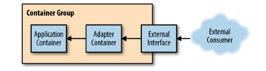
The first single-node pattern is the sidecar pattern. The sidecar pattern is a single node pattern made up of two containers. The first is the application container. It contains the core logic for the application. Without this container, the application would not exist. In addition to the application container, there is a sidecar container. The role of the sidecar is to augment and improve the application container, often without the application container’s knowledge. In its simplest form, a sidecar container can be used to add functionality to a container that might otherwise be difficult to improve. Sidecar containers are coscheduled onto the same machine via an atomic container group, such as the pod API object in Kubernetes. In addition to being scheduled on the same machine, the application container and sidecar container share a number of resources, including parts of the filesystem, hostname and network, and many other namespaces.
Ambassadors
An ambassador container brokers interactions between the application container and the rest of the world. As with other single-node patterns, the two containers are tightly linked in a symbiotic pairing that is scheduled to a single machine.
It allows for easier management and maintenance of communication between services, and can extend the networking capabilities of legacy applications.
Put client frameworks and libraries into an external process that acts as a proxy between your application and external services. Deploy the proxy on the same host environment as your application to allow control over routing, resiliency, security features, and to avoid any host-related access restrictions. You can also use the ambassador pattern to standardize and extend instrumentation. The proxy can monitor performance metrics such as latency or resource usage, and this monitoring happens in the same host environment as the application.
The Ambassador Pattern and the Sidecar Pattern can seem similar because they both involve deploying additional containers alongside the main application container. However, they serve different purposes and are used in different contexts:
Sidecar Pattern: In this pattern, an additional container (the sidecar) is deployed alongside the main application container. The sidecar extends or enhances the functionality of the main container without changing the application itself. For example, a sidecar container might handle logging or monitoring.
Ambassador Pattern: This pattern is similar to the sidecar pattern, but in the ambassador pattern, every interaction to the outside world goes through the ambassador container. The ambassador acts as a proxy for outgoing network traffic from the main container. This means that the main application container cannot contact the outside world without the ambassador. For example, an ambassador container might handle network requests to a database or other external service.
Here are some use cases for both the Ambassador Pattern and the Sidecar Pattern:
Ambassador Pattern Use Cases:
- Sharding: The Ambassador Pattern can be used to implement sharding. The ambassador can route requests to different databases based on the sharding logic.
- Network Proxy: The ambassador can act as a network proxy, handling all network requests for the main application. This is useful when the main application needs to communicate with external services.
- Monitoring and Logging: The ambassador can handle tasks such as monitoring and logging, offloading these tasks from the main application.
Sidecar Pattern Use Cases:
- Logging: A sidecar container can be used to handle logging. This allows the main application to focus on its core functionality, while the sidecar handles the logging.
- Monitoring: Similar to logging, a sidecar can also handle monitoring. This can include monitoring the performance of the main application.
- Security: A sidecar can handle security-related tasks, such as encryption and authentication.
Adapters
The adapter container is used to modify the interface of the application container so that it conforms to some predefined interface that is expected of all applications. For example, an adapter might ensure that an application implements a consistent monitoring interface. Or it might ensure that log files are always written to stdout or any number of other conventions.
Single-node examples illustrate the power of this pattern:
Monitoring: Applications often speak different dialects of data metrics. An adapter can translate them into a common language for a central monitoring tool.
Logging: Applications might write their tales in various formats or locations. An adapter can unify their logs before sending them to a central storyteller.
Health Check Adapter: Create an adapter component dedicated to performing health checks.
Serving Patterns
The previous we described patterns for grouping collections of containers that are scheduled on the same machine. These groups are tightly coupled, symbiotic systems. They depend on local, shared resources like disk, network interface, or interprocess communications. Such collections of containers are important patterns, but they are also building blocks for larger systems.
Reliability, scalability, and separation of concerns dictate that real-world systems are built out of many different components, spread across multiple machines. In contrast to single-node patterns, the multi-node distributed patterns are more loosely coupled. While the patterns dictate patterns of communication between the components, this communication is based on network calls. Furthermore, many calls are issued in parallel, and systems coordinate via loose synchronization rather than tight constraints.
Introduction to Microservices
Recently, the term microservices has become a buzzword for describing multi-node distributed software architectures. Microservices describe a system built out of many different components running in different processes and communicating over defined APIs. Microservices stand in contrast to monolithic systems, which tend to place all of the functionality for a service within a single, tightly coordinated application.
There are numerous benefits to the microservices approach, most of them are centered around reliability and agility. Microservices break down an application into small pieces, each focused on providing a single service. This reduced scope enables each service to be built and maintained by a single “two pizza” team. Reduced team size also reduces the overhead associated with keeping a team focused and moving in one direction.
Additionally, the introduction of formal APIs in between different microservices decouples the teams from one another and provides a reliable contract between the different services. This formal contract reduces the need for tight synchronization among the teams because the team providing the API understands the surface area that it needs to keep stable, and the team consuming the API can rely on a stable service without worrying about its details. This decoupling enables teams to independently manage their code and release schedules, which in turn improves each team’s ability to iterate and improve their code.
But of course there are downsides to the microservices approach to system design as well. The two foremost disadvantages are that because the system has become more loosely coupled, debugging the system when failures occur is significantly more difficult. You can no longer simply load a single application into a debugger and determine what went wrong. Any errors are the byproducts of a large number of systems often running on different machines. This environment is quite challenging to reproduce in a debugger. As a corollary, microservices-based systems are also difficult to design and architect. A microservices-based system uses multiple methods of communicating between services; different patterns (e.g., synchronous, asynchronous, message-passing, etc.); and multiple different patterns of coordination and control among the services.
These challenges are the motivation for distributed patterns. If a microservices architecture is made up of well-known patterns, then it is easier to design because many of the design practices are specified by the patterns. Additionally, patterns make the systems easier to debug because they enable developers to apply lessons learned across a number of different systems that use the same patterns.
Replicated Load-Balanced Services
The simplest distributed pattern, and one that most are familiar with, is a replicated load-balanced service. In such a service, every server is identical to every other server and all are capable of supporting traffic. The pattern consists of a scalable number of servers with a load balancer in front of them. The load balancer is typically either completely round-robin or uses some form of session stickiness.
Stateless Services
Stateless services are ones that don’t require saved state to operate correctly. In the simplest stateless applications, even individual requests may be routed to separate instances of the service.
Stateless systems are replicated to provide redundancy and scale. No matter how small your service is, you need at least two replicas to provide a service with a “highly available” service level agreement (SLA). To understand why this is true, consider trying to deliver a three-nines (99.9% availability). In a three-nines service, you get 1.4 minutes of downtime per day (24 × 60 × 0.001). Assuming that you have a service that never crashes, that still means you need to be able to do a software upgrade in less than 1.4 minutes in order to hit your SLA with a single instance. And that’s assuming that you do daily software rollouts. If your team is really embracing continuous delivery and you’re pushing a new version of software every hour, you need to be able to do a software rollout in 3.6 seconds to achieve your 99.9% uptime SLA with a single instance. Any longer than that and you will have more than 0.01% downtime from those 3.6 seconds.
Of course, instead of all of that work, you could just have two replicas of your service with a load balancer in front of them. As services grow larger, they are also replicated to support additional users. Horizontally scalable systems handle more and more users by adding more replicas.
Simply replicating your service and adding a load balancer is only part of a complete pattern for stateless replicated serving. When designing a replicated service, it is equally important to build and deploy a readiness probe to inform the load balancer. We have discussed how health probes can be used by a container orchestration system to determine when an application needs to be restarted. In contrast, a readiness probe determines when an application is ready to serve user requests. The reason for the differentiation is that many applications require some time to become initialized before they are ready to serve. They may need to connect to databases, load plugins, or download serving files from the network. In all of these cases, the containers are alive, but they are not ready. When building an application for a replicated service pattern, be sure to include a special URL that implements this readiness check.
Session Tracked Services
The previous examples of the stateless replicated pattern routed requests from all users to all replicas of a service. While this ensures an even distribution of load and fault tolerance, it is not always the preferred solution. Often there are reasons for wanting to ensure that a particular user’s requests always end up on the same machine. Sometimes this is because you are caching that user’s data in memory, so landing on the same machine ensures a higher cache hit rate. Sometimes it is because the interaction is long-running in nature, so some amount of state is maintained between requests. Regardless of the reason, an adaption of the stateless replicated service pattern is to use session tracked services, which ensure that all requests for a single user map to the same replica,
Generally speaking, this session tracking is performed by hashing the source and destination IP addresses and using that key to identify the server that should service the requests. So long as the source and destination IP addresses remain constant, all requests are sent to the same replica.
IP-based session tracking works within a cluster (internal IPs) but generally doesn’t work well with external IP addresses because of network address translation (NAT). For external session tracking, application-level tracking (e.g., via cookies) is preferred.
Often, session tracking is accomplished via a consistent hashing function. The benefit of a consistent hashing function becomes evident when the service is scaled up or down. Obviously, when the number of replicas changes, the mapping of a particular user to a replica may change. Consistent hashing functions minimize the number of users that actually change which replica they are mapped to, reducing the impact of scaling on your application.
Application-Layer Replicated Services
In all of the preceding examples, the replication and load balancing takes place in the network layer of the service. The load balancing is independent of the actual protocol that is being spoken over the network, beyond TCP/IP. However, many applications use HTTP as the protocol for speaking with each other, and knowledge of the application protocol that is being spoken enables further refinements to the replicated stateless serving pattern for additional functionality.
Introducing a Caching Layer
Sometimes the code in your stateless service is still expensive despite being stateless. It might make queries to a database to service requests or do a significant amount of rendering or data mixing to service the request. In such a world, a caching layer can make a great deal of sense. A cache exists between your stateless application and the end-user request. The simplest form of caching for web applications is a caching web proxy. The caching proxy is simply an HTTP server that maintains user requests in memory state. If two users request the same web page, only one request will go to your backend; the other will be serviced out of memory in the cache.
Deploying Your Cache
The simplest way to deploy the web cache is alongside each instance of your web server using the sidecar pattern.
Though this approach is simple, it has some disadvantages, namely that you will have to scale your cache at the same scale as your web servers. This is often not the approach you want. For your cache, you want as few replicas as possible with lots of resources for each replica (e.g., rather than 10 replicas with 1 GB of RAM each, you’d want two replicas with 5 GB of RAM each). To understand why this is preferable, consider that every page will be stored in every replica. With 10 replicas, you will store every page 10 times, reducing the overall set of pages that you can keep in memory in the cache. This causes a reduction in the hit rate, the fraction of the time that a request can be served out of cache, which in turn decreases the utility of the cache. Though you do want a few large caches, you might also want lots of small replicas of your web servers. Many languages (e.g., NodeJS) can really only utilize a single core, and thus you want many replicas to be able to take advantages of multiple cores, even on the same machine. Therefore, it makes the most sense to configure your caching layer as a second stateless replicated serving tier above your web-serving tier.
Expanding the Caching Layer
Now that we have inserted a caching layer into our stateless, replicated service, let’s look at what this layer can provide beyond standard caching. HTTP reverse proxies like Varnish are generally pluggable and can provide a number of advanced features that are useful beyond caching.
Rate Limiting and Denial-of-Service Defense
Few of us build sites with the expectation that we will encounter a denial-of-service attack. But as more and more of us build APIs, a denial of service can come simply from a developer misconfiguring a client or a site-reliability engineer accidentally running a load test against a production installation. Thus, it makes sense to add general denial-of-service defense via rate limiting to the caching layer. Most HTTP reverse proxies like Varnish have capabilities along this line. In particular, Varnish has a throttle module that can be configured to provide throttling based on IP address and request path, as well as whether or not a user is logged in.
If you are deploying an API, it is generally a best practice to have a relatively small rate limit for anonymous access and then force users to log in to obtain a higher rate limit. Requiring a login provides auditing to determine who is responsible for the unexpected load, and also offers a barrier to would-be attackers who need to obtain multiple identities to launch a successful attack.
When a user hits the rate limit, the server will return the 429 error code indicating that too many requests have been issued. However, many users want to understand how many requests they have left before hitting that limit. To that end, you will likely also want to populate an HTTP header with the remaining-calls information. Though there isn’t a standard header for returning this data, many APIs return some variation of X-RateLimit-Remaining.
SSL Termination
In addition to performing caching for performance, one of the other common tasks performed by the edge layer is SSL termination. Even if you plan on using SSL for communication between layers in your cluster, you should still use different certificates for the edge and your internal services. Indeed, each individual internal service should use its own certificate to ensure that each layer can be rolled out independently. Unfortunately, the Varnish web cache can’t be used for SSL termination, but fortunately, the nginx application can. Thus we want to add a third layer to our stateless application pattern, which will be a replicated layer of nginx servers that will handle SSL termination for HTTPS traffic and forward traffic on to our Varnish cache. HTTP traffic continues to travel to the Varnish web cache, and Varnish forwards traffic on to our web application.
Sharded Services
In the previous chapter, we saw the value of replicating stateless services for reliability, redundancy, and scaling. This chapter considers sharded services. With the replicated services that we introduced in the preceding chapter, each replica was entirely homogeneous and capable of serving every request. In contrast to replicated services, with sharded services, each replica, or shard, is only capable of serving a subset of all requests. A load-balancing node, or root, is responsible for examining each request and distributing each request to the appropriate shard or shards for processing.
Replicated services are generally used for building stateless services, whereas sharded services are generally used for building stateful services. The primary reason for sharding the data is because the size of the state is too large to be served by a single machine. Sharding enables you to scale a service in response to the size of the state that needs to be served.
Sharded Caching
To completely illustrate the design of a sharded system, this section provides a deep dive into the design of a sharded caching system. A sharded cache is a cache that sits between the user requests and the actually frontend implementation.
we discussed how an ambassador could be used to distribute data to a sharded service. This section discusses how to build that service. When designing a sharded cache, there are a number of design aspects to consider:
• Why you might need a sharded cache
• The role of the cache in your architecture
• Replicated, sharded caches
• The sharding function
Why You Might Need a Sharded Cache
As was mentioned in the introduction, the primary reason for sharding any service is to increase the size of the data being stored in the service. To understand how this helps a caching system, imagine the following system: Each cache has 10 GB of RAM available to store results, and can serve 100 requests per second (RPS). Suppose then that our service has a total of 200 GB possible results that could be returned, and an expected 1,000 RPS. Clearly, we need 10 replicas of the cache in order to satisfy 1,000 RPS (10 replicas × 100 requests per second per replica). The simplest way to deploy this service would be as a replicated service, as described in the previous chapter. But deployed this way, the distributed cache can only hold a maximum of 5% (10 GB/200 GB) of the total data set that we are serving. This is because each cache replica is independent, and thus each cache replica stores roughly the exact same data in the cache. This is great for redundancy, but pretty terrible for maximizing memory utilization. If instead, we deploy a 10-way sharded cache, we can still serve the appropri‐ate number of RPS (10 × 100 is still 1,000), but because each cache serves a completely unique set of data, we are able to store 50% (10 × 10 GB/200 GB) of the total data set. This tenfold increase in cache storage means that the memory for the cache is much better utilized, since each key exists only in a single cache.
The Role of the Cache in System Performance
we discussed how caches can be used to optimize end-user performance and latency, but one thing that wasn’t covered was the criticality of the cache to your application’s performance, reliability, and stability. Put simply, the important question for you to consider is: If the cache were to fail, what would the impact be for your users and your service? When we discussed the replicated cache, this question was less relevant because the cache itself was horizontally scalable, and failures of specific replicas would only lead to transient failures. Likewise, the cache could be horizontally scaled in response to increased load without impacting the end user. This changes when you consider sharded caches. Because a specific user or request is always mapped to the same shard, if that shard fails, that user or request will always miss the cache until the shard is restored. Given the nature of a cache as transient data, this miss is not inherently a problem, and your system must know how to recalculate the data. However, this recalculation is inherently slower than using the cache directly, and thus it has performance implications for your end users. The performance of your cache is defined in terms of its hit rate. The hit rate is the percentage of the time that your cache contains the data for a user request. Ultimately, the hit rate determines the overall capacity of your distributed system and affects the overall capacity and performance of your system. Imagine, if you will, that you have a request-serving layer that can handle 1,000 RPS. After 1,000 RPS, the system starts to return HTTP 500 errors to users. If you place a cache with a 50% hit rate in front of this request-serving layer, adding this cache increases your maximum RPS from 1,000 RPS to 2,000 RPS. To understand why this is true, you can see that of the 2,000 inbound requests, 1,000 (50%) can be serviced by the cache, leaving 1,000 requests to be serviced by your serving layer. In this instance, the cache is fairly critical to your service, because if the cache fails, then the serving layer will be overloaded and half of all your user requests will fail. Given this, it likely makes sense to rate your service at a maximum of 1,500 RPS rather than the full 2,000 RPS. If you do this, then you can sustain a failure of half of your cache replicas and still keep your service stable. But the performance of your system isn’t just defined in terms of the number of requests that it can process. Your system’s end-user performance is defined in terms of the latency of requests as well. A result from a cache is generally significantly faster than calculating that result from scratch. Consequently, a cache can improve the speed of requests as well as the total number of requests processed. To see why this is true, imagine that your system can serve a request from a user in 100 milliseconds. You add a cache with a 25% hit rate that can return a result in 10 milliseconds. Thus, the average latency for a request in your system is now 77.5 milliseconds. Unlike maximum requests per second, the cache simply makes your requests faster, so there is somewhat less need to worry about the fact that requests will slow down if the cache fails or is being upgraded. However, in some cases, the performance impact can cause too many user requests to pile up in request queues and ultimately time out. It’s always recommended that you load test your system both with and without caches to understand the impact of the cache on the overall performance of your system. Finally, it isn’t just failures that you need to think about. If you need to upgrade or redeploy a sharded cache, you can not just deploy a new replica and assume it will take the load. Deploying a new version of a sharded cache will generally result in temporarily losing some capacity. Another, more advanced option is to replicate your shards.
Replicated, Sharded Caches
Sometimes your system is so dependent on a cache for latency or load that it is not acceptable to lose an entire cache shard if there is a failure or you are doing a rollout. Alternatively, you may have so much load on a particular cache shard that you need to scale it to handle the load. For these reasons, you may choose to deploy a sharded, replicated service. A sharded, replicated service combines the replicated service pattern described in the previous chapter with the sharded pattern described in previous sections. In a nutshell, rather than having a single server implement each shard in the cache, a replicated service is used to implement each cache shard. This design is obviously more complicated to implement and deploy, but it has several advantages over a simple sharded service. Most importantly, by replacing a single server with a replicated service, each cache shard is resilient to failures and is always present during failures. Rather than designing your system to be tolerant to performance degradation resulting from cache shard failures, you can rely on the performance improvements that the cache provides. Assuming that you are willing to overprovision shard capacity, this means that it is safe for you to do a cache rollout during peak traffic, rather than waiting for a quiet period for your service. Additionally, because each replicated cache shard is an independent replicated service, you can scale each cache shard in response to its load; this sort of “hot sharding” is discussed at the end of this chapter.
An Examination of Sharding Functions
So far we’ve discussed the design and deployment of both simple sharded and replicated sharded caches, but we haven’t spent very much time considering how traffic is routed to different shards. Consider a sharded service where you have 10 independent shards. Given some specific user request Req, how do you determine which shard S in the range from zero to nine should be used for the request? This mapping is the responsibility of the sharding function. A sharding function is very similar to a hashing function, which you may have encountered when learning about hashtable data structures. Indeed, a bucket-based hashtable could be considered an example of a sharded service. Given both Req and Shard, then the role of the sharding function is to relate them together, specifically:
Shard = ShardingFunction(Req)
Commonly, the sharding function is defined using a hashing function and the modulo (%) operator. Hashing functions are functions that transform an arbitrary object into an integer hash. The hash function has two important characteristics for our sharding:
Determinism The output should always be the same for a unique input.
Uniformity The distribution of outputs across the output space should be equal.
For our sharded service, determinism and uniformity are the most important characteristics. Determinism is important because it ensures that a particular request R always goes to the same shard in the service. Uniformity is important because it ensures that load is evenly spread between the different shards.
Fortunately for us, modern programming languages include a wide variety of highquality hash functions. However, the outputs of these hash functions are often significantly larger than the number of shards in a sharded service. Consequently, we use the modulo operator (%) to reduce a hash function to the appropriate range. Returning to our sharded service with 10 shards, we can see that we can define our sharding function as:
Shard = hash(Req) % 10
If the output of the hash function has the appropriate properties in terms of determinism and uniformity, those properties will be preserved by the modulo operator.
Selecting a Key
Given this sharding function, it might be tempting to simply use the hashing function that is built into the programming language, hash the entire object, and call it a day. The result of this, however, will not be a very good sharding function. To understand this, consider a simple HTTP request that contains three things:
• The time of the request
• The source IP address from the client
• The HTTP request path (e.g., /some/page.html)
If we use a simple object-based hashing function, shard(request), then it is clear that {12:00, 1.2.3.4, /some/file.html} has a different shard value than {12:01, 5.6.7.8, /some/file.html}. The output of the sharding function is different because the client’s IP address and the time of the request are different between the two requests. But of course, in most cases, the IP address of the client and the time of the request don’t impact the response to the HTTP request. Consequently, instead of hashing the entire request object, a much better sharding function would be shard(request.path). When we use request.path as the shard key, then we map both requests to the same shard, and thus the response to one request can be served out of the cache to service the other.
Of course, sometimes client IP is important to the response that is returned from the frontend. For example, client IP may be used to look up the geographic region that the user is located in, and different content (e.g., different languages) may be returned to different IP addresses. In such cases, the previous sharding function shard(request.path) will actually result in errors, since a cache request from a French IP address may be served a result page from the cache in English. In such cases, the cache function is too general, as it groups together requests that do not have identical responses.
Given this problem, it would be tempting then to define our sharding function as shard(request.ip, request.path), but this sharding function has problems as well. It will cause two different French IP addresses to map to different shards, thus resulting in inefficient sharding. This shard function is too specific, as it fails to group together requests that are identical. A better sharding function for this situation would be:
shard(country(request.ip), request.path)
This first determines the country from the IP address, and then uses that country as part of the key for the sharding function. Thus multiple requests from France will be routed to one shard, while requests from the United States will be routed to a different shard. Determining the appropriate key for your sharding function is vital to designing your sharded system well. Determining the correct shard key requires an understanding of the requests that you expect to see.
Consistent Hashing Functions
Setting up the initial shards for a new service is relatively straightforward: you set up the appropriate shards and the roots to perform the sharding, and you are off to the races. However, what happens when you need to change the number of shards in your sharded service? Such “re-sharding” is often a complicated process. To understand why this is true, consider the sharded cache previously examined. Certainly, scaling the cache from 10 to 11 replicas is straightforward to do with a con‐tainer orchestrator, but consider the effect of changing the scaling function from hash(Req) % 10 to hash(Req) % 11. When you deploy this new scaling function, a large number of requests are going to be mapped to a different shard than the one they were previously mapped to. In a sharded cache, this is going to dramatically increase your miss rate until the cache is repopulated with responses for the new requests that have been mapped to that cache shard by the new sharding function. In the worst case, rolling out a new sharding function for your sharded cache will be equivalent to a complete cache failure.
To resolve these kinds of problems, many sharding functions use consistent hashing functions. Consistent hashing functions are special hash functions that are guaranteed to only remap # keys / # shards, when being resized to # shards. For example, if we use a consistent hashing function for our sharded cache, moving from 10 to 11 shards will only result in remapping < 10% (K / 11) keys. This is dramatically better than losing the entire sharded service.
Sharded, Replicated Serving
Most of the examples in this chapter so far have described sharding in terms of cache serving. But, of course, caches are not the only kinds of services that can benefit from sharding. Sharding is useful when considering any sort of service where there is more data than can fit on a single machine. In contrast to previous examples, the key and sharding function are not a part of the HTTP request, but rather some context for the user. For example, consider implementing a large-scale multi-player game. Such a game world is likely to be far too large to fit on a single machine. However, players who are distant from each other in this virtual world are unlikely to interact. Consequently, the world of the game can be sharded across many different machines. The sharding function is keyed off of the player’s location so that all players in a particular location land on the same set of servers.
Hot Sharding Systems
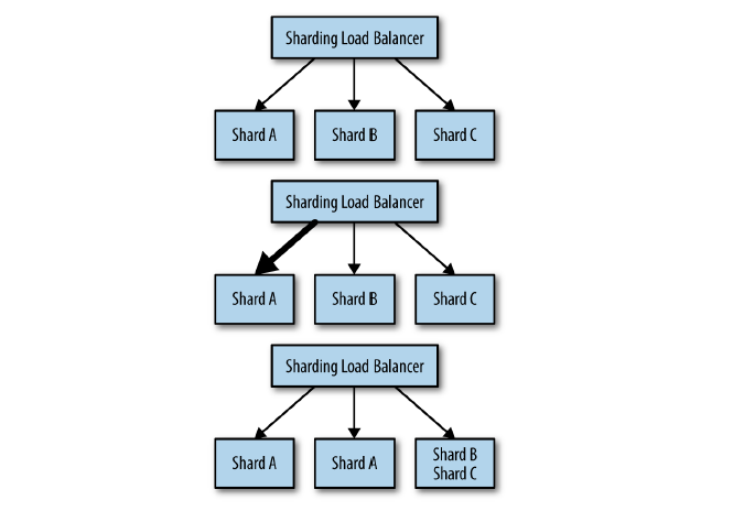
Ideally the load on a sharded cache will be perfectly even, but in many cases this isn’t true and “hot shards” appear because organic load patterns drive more traffic to one particular shard. As an example of this, consider a sharded cache for a user’s photos; when a particular photo goes viral and suddenly receives a disproportionate amount of traffic, the cache shard containing that photo will become “hot.” When this happens, with a replicated, sharded cache, you can scale the cache shard to respond to the increased load. Indeed, if you set up autoscaling for each cache shard, you can dynamically grow and shrink each replicated shard as the organic traffic to your service shifts around. An illustration of this process is shown in Figure 6-3. Initially the sharded service receives equal traffic to all three shards. Then the traffic shifts so that Shard A is receiving four times as much traffic as Shard B and Shard C. The hot sharding system moves Shard B to the same machine as Shard C, and replicates Shard A to a second machine. Traffic is now, once again, equally shared between replicas.
Like replicated and sharded systems, the scatter/gather pattern is a tree pattern with a root that distributes requests and leaves that process those requests. However, in contrast to replicated and sharded systems, with scatter/gather requests are simultaneously farmed out to all of the replicas in the system. Each replica does a small amount of processing and then returns a fraction of the result to the root. The root server then combines the various partial results together to form a single complete response to the request and then sends this request back out to the client.
Scatter/gather is quite useful when you have a large amount of mostly independent processing that is needed to handle a particular request. Scatter/gather can be seen as sharding the computation necessary to service the request, rather than sharding the data (although data sharding may be part of it as well).
Scatter/Gather with Root Distribution
The simplest form of scatter/gather is one in which each leaf is entirely homogenous but the work is distributed to a number of different leaves in order to improve the performance of the request. This pattern is equivalent to solving an “embarassingly parallel” problem. The problem can be broken up into many different pieces and each piece can be put back together with all of the other pieces to form a complete answer. To understand this in more concrete terms, imagine that you need to service a user request R and it takes one minute for a single core to produce the answer A to this request. If we program a multi-threaded application, we can parallelize this request on a single machine by using multiple cores. Given this approach and a 30 core processor (yes, typically it would be a 32 core processor, but 30 makes the math cleaner), we can reduce the time that it takes to process a single request down to 2 seconds (60 seconds of computation split across 30 threads for computation is equal to 2 seconds). But even two seconds is pretty slow to service a user’s web request. Additionally, truly achieving a completely parallel speed up on a single process is going to be tricky as things like memory, network, or disk bandwidth start to become the bottleneck. Instead of parallelizing an application across cores on a single machine, we can use the scatter/gather pattern to parallelize requests across multiple processes on many different machines. In this way, we can improve our overall latency requests, since we are no longer bound by the number of cores we can get on a single machine, as well as ensure that the bottleneck in our process continues to be CPU, since the memory, network, and disk bandwidth are all spread across a number of different machines. Additionally, because every machine in the scatter/gather tree is capable of handling every request, the root of the tree can dynamically dispatch load to different nodes at different times depending on their responsiveness. If, for some reason, a particular leaf node is responding more slowly than other machines (e.g., it has a noisy neighbor process that is interfering with resources), then the root can dynamically redistribute load to assure a fast response.
Hands On: Distributed Document Search
To see an example of scatter/gather in action, consider the task of searching across a large database of documents for all documents that contain the words “cat” and “dog.” One way to perform this search would be to open up all of the documents, read through the entire set, searching for the words in each document, and then return to the user the set of documents that contain both words. As you might imagine, this is quite a slow process because it requires opening and reading through a large number of files for each request. To make request processing faster, you can build an index. The index is effectively a hashtable, where the keys are individual words (e.g., “cat”) and the values are a list of documents containing that word. Now, instead of searching through every document, finding the documents that match any one word is as easy as doing a lookup in this hashtable. However, we have lost one important ability. Remember that we were looking for all documents that contained “cat” and “dog.” Since the index only has single words, not conjunctions of words, we still need to find the documents that contain both words. Luckily, this is just an intersection of the sets of documents returned for each word. Given this approach, we can implement this document search as an example of the scatter/gather pattern. When a request comes in to the document search root, it parses the request and farms out two leaf machines (one for the word “cat” and one for the word “dog”). Each of these machines returns a list of documents that match one of the words, and the root node returns the list of documents containing both “cat” and “dog.”
Scatter/Gather with Leaf Sharding
While applying the replicated data scatter/gather pattern allows you to reduce the processing time required for handling user requests, it doesn’t allow you to scale beyond an amount of data that can be held in the memory or disk of a single machine. Much like the replicated serving pattern that was previously described, it is simple to build a replicated scatter/gather system. But at a certain data size, it is necessary to introduce sharding in order to build a system that can hold more data than can be stored on a single machine. Previously, when sharding was introduced to scale replicated systems, the sharding was done at a per-request level. Some part of the request was used to determine where the request was sent. That replica then handled all of the processing for the request and the response was handed back to the user. Instead, with scatter/gather sharding, the request is sent to all of the leaf nodes (or shards) in the system. Each leaf node processes the request using the data that it has loaded in its shard. This partial response is then returned to the root node that requested data, and that root node merges all of the responses together to form a comprehensive response for the user. As a concrete example of this sort of architecture, consider implementing search across a very large document set (all patents in the world, for example); in such a case, the data is too large to fit in the memory of a single machine, so instead the data is sharded across multiple replicas. For example, patents 0-100,000 might be on the first machine, 100,001-200,000 on the next machine, and so forth. (Note that this is not actually a good sharding scheme since it will continually force us to add new shards as new patents are registered. In practice, we’d likely use the patent number modulo the total number of shards.) When a user submits a request to find a particular word (e.g., “rockets”) in all of the patents in the index, that request is sent to each shard, which searches through it’s patent shard for patents which match the word in the query. Any matches that are found are returned to the root node in response to the shard request. The root node then collates all of these responses together into a single response that contains all the patents that match the particular word.
The previous example scattered the different term requests across the cluster, but this only works if all of the documents are present on all of the machines in the scatter/ gather tree. If there is not enough room for all of the documents in all of the leaves in the tree, then sharding must be used to put different sets of documents onto different leaves. This means that when a user makes a request for all documents that match the words “cat” and “dog,” the request is actually sent out to every leaf in the scatter/gather system. Each leaf node returns the set of documents that it knows about that matches “cat” and “dog.” Previously, the root node was responsible for performing the intersection of the two sets of documents returned for two different words. In the sharded case, the root node is responsible for generating the union of all of the documents returned by all of the different shards and returning this complete set of documents back up to the user.
Choosing the Right Number of Leaves
It might seem that in the scatter/gather pattern, replicating out to a very large number of leaves would always be a good idea. You parallelize your computation and consequently reduce the clock time required to process any particular request. However, increased parallelization comes at a cost, and thus choosing the right number of leaf nodes in the scatter/gather pattern is critical to designing a performant distributed system. To understand how this can happen, it’s worth considering two things. The first is that processing any particular request has a certain amount of overhead. This is the time spent parsing a request, sending HTTP across the wire, and so forth. In general, the overhead due to system request handling is constant and significantly less than the time spent in user code processing the request. Consequently, this overhead can generally be ignored when assessing the performance of the scatter/gather pattern. However, it is important to understand that the cost of this overhead scales with the number of leaf nodes in the scatter/gather pattern. Thus, even though it is low cost, as parallelization continues, this overhead eventually dominates the compute cost of your business logic. This means that the gains of parallelization are asymptotic. In addition to the fact that adding more leaf nodes may not actually speed up processing, scatter/gather systems also suffer from the “straggler” problem. To understand how this works, it is important to remember that in a scatter/gather system, the root node waits for requests from all of the leaf nodes to return before sending a response back to the end user. Since data from every leaf node is required, the overall time it takes to process a user request is defined by the slowest leaf node that sends a response. To understand the impact of this, imagine that we have a service that has a 99th percentile latency of 2 seconds. This means that on average one request out of every 100 has a latency of 2 seconds, or put another way, there is a 1% chance that a request will take 2 seconds. This may be totally acceptable at first glance: a single user out of 100 has a slow request. However, consider how this actually works in a scatter/ gather system. Since the time of the user request is defined by the slowest response, we need to consider not a single request but all requests scattered out to the various leaf nodes. Let’s see what happens when we scatter out to five leaf nodes.
In this situation, there is a 5% chance that one of these five scatter requests has a latency of 2 seconds (0.99 × 0.99 × 0.99 × 0.99 × 0.99 == 0.95). This means that our 99th percentile latency for individual requests becomes a 95th percentile latency for our complete scatter/gather system. And it only gets worse from there: if we scatter out to 100 leaves, then we are more or less guaranteeing that our overall latency for all requests will be 2 seconds.
Scaling Scatter/Gather for Reliability and Scale
Of course, just as with a sharded system, having a single replica of a sharded scatter/ gather system is likely not the desirable design choice. A single replica means that if it fails, all scatter/gather requests will fail for the duration that the shard is unavailable because all requests are required to be processed by all leaf nodes in the scatter/gather pattern. Likewise, upgrades will take out a percentage of your shards, so an upgrade while under user-facing load is no longer possible. Finally, the computational scale of your system will be limited by the load that any single node is capable of achieving. Ultimately, this limits your scale, and as we have seen in previous sections, you cannot simply increase the number of shards in order to improve the computational power of a scatter/gather pattern.
Given these challenges of reliability and scale, the correct approach is to replicate each of the individual shards so that instead of a single instance at each leaf node, there is a replicated service that implements each leaf shard.
Built this way, each leaf request from the root is actually load balanced across all healthy replicas of the shard. This means that if there are any failures, they won’t result in a user-visible outage for your system. Likewise, you can safely perform an upgrade under load, since each replicated shard can be upgraded one replica at a time. Indeed, you can perform the upgrade across multiple shards simultaneously, depending on how quickly you want to perform the upgrade.
Functions and Event-Driven Processing
So far, we have examined design for systems with long-running computation. The servers that handle user requests are always up and running. This pattern is the right one for many applications that are under heavy load, keep a large amount of data in memory, or require some sort of background processing. However, there is a class of applications that might only need to temporarily come into existence to handle a single request, or simply need to respond to a specific event. This style of request or event-driven application design has flourished recently as large-scale public cloud providers have developed function-as-a-service (FaaS) products. More recently, FaaS implementations have also emerged running on top of cluster orchestrators in private cloud or physical environments. This chapter describes emerging architectures for this new style of computing. In many cases, FaaS is a component in a broader architecture rather than a complete solution.
Oftentimes, FaaS is referred to as serverless computing. And while this is true (you don’t see the servers in FaaS) it’s worth differentiating between event-driven FaaS and the broader notion of serverless computing. Indeed, serverless computing can apply to a wide variety of computing services; for example, a multi-tenant container orchestrator (container-as-a-service) is serverless but not eventdriven. Conversely, an open source FaaS running on a cluster of physical machines that you own and administer is event-driven but not serverless. Understanding this distinction enables you to determine when event-driven, serverless, or both is the right choice for your application.
Determining When FaaS Makes Sense
As with many tools for developing a distributed system, it can be tempting to see a particular solution like event-driven processing as a universal hammer. However, the truth is that it is best suited to a particular set of problems. Within a particular context it is a powerful tool, but stretching it to fit all applications or systems will lead to overly complicated, brittle designs. Especially since FaaS is such a new computing tool, before discussing specific design patterns, it is worth discussing the benefits, limitations, and optimal situations for employing event-driven computing.
The Benefits of FaaS
The benefits of FaaS are primarily for the developer. It dramatically simplifies the distance from code to running service. Because there is no artifact to create or push beyond the source code itself, FaaS makes it simple to go from code on a laptop or web browser to running code in the cloud. Likewise, the code that is deployed is managed and scaled automatically. As more traffic is loaded onto the service, more instances of the function are created to handle that increase in traffic. If a function fails due to application or machine failures, it is automatically restarted on some other machine. Finally, much like containers, functions are an even more granular building block for designing distributed systems. Functions are stateless and thus any system you build on top of functions is inherently more modular and decoupled than a similar system built into a single binary. But, of course, this is also the challenge of developing systems in FaaS. The decoupling is both a strength and a weakness. The following section describes some of the challenges that come from developing systems using FaaS.
The Challenges of FaaS
As described in the previous section, developing systems using FaaS forces you to strongly decouple each piece of your service. Each function is entirely independent. The only communication is across the network, and each function instance cannot have local memory, requiring all states to be stored in a storage service. This forced decoupling can improve the agility and speed with which you can develop services, but it can also significantly complicate the operations of the same service. In particular, it is often quite difficult to obtain a comprehensive view of your service, determine how the various functions integrate with one another, and understand when things go wrong, and why they go wrong. Additionally, the request-based and serverless nature of functions means that certain problems are quite difficult to detect.
Now consider what happens when a request comes into any of these functions: it kicks off an infinite loop that only terminates when the original request times out (and possibly not even then) or when you run out of money to pay for requests in the system. Obviously, the above example is quite contrived, but it is actually quite difficult to detect in your code. Since each function is radically decoupled from the other functions, there is no real representation of the dependencies or interactions between different functions. These problems are not unsolvable, and I expect that as FaaSs mature, more analysis and debugging tools will provide a richer experience to understand how and why an application comprised of FaaS is performing the way that it does. For now, when adopting FaaS, you must be vigilant to adopt rigorous monitoring and alerting for how your system is behaving so that you can detect situations and correct them before they become significant problems. Of course, the complexity introduced by monitoring flies somewhat in the face of the simplicity of deploying to FaaS, which is friction that your developers must overcome.
The Need for Background Processing
FaaS is inherently an event-based application model. Functions are executed in response to discrete events that occur and trigger the execution of the functions. Additionally, because of the serverless nature of the implementation of theses services, the runtime of any particular function instance is generally time bounded. This means that FaaS is usually a poor fit for situations that require processing. Examples of such background processing might be transcoding a video, compressing log files, or other sorts of low-priority, long-running computations. In many cases, it is possible to set up a scheduled trigger that synthetically generates events in your functions on a particular schedule. Though this is a good fit for responding to temporal events (e.g., firing a text-message alarm to wake someone up), it is still not sufficient infrastructure for generic background processing. To achieve that, you need to launch your code in an environment that supports long-running processes. And this generally means switching to a pay-per-consumption rather than pay-per-request model for the parts of your application that do background processing.
The Need to Hold Data in Memory
In addition to the operational challenges, there are some architectural limitations that make FaaS ill-suited for some types of applications. The first of these limitations is the need to have a significant amount of data loaded into memory in order to process user requests. There are a variety of services (e.g., serving a search index of documents) that require a great deal of data to be loaded in memory in order to service user requests. Even with a relatively fast storage layer, loading such data can take significantly longer than the desired time to service a user request. Because with FaaS, the function itself may be dynamically spun up in response to a user request while the user is waiting, the need to load a lot of detail may significantly impact the latency that the user perceives while interacting with your service. Of course, once your FaaS has been created, it may handle a large number of requests, so this loading cost can be amortized across a large number of requests. But if you have a sufficient number of requests to keep a function active, then it’s likely you are overpaying for the requests you are processing.
The Costs of Sustained Request-Based Processing
The cost model of public cloud FaaS is based on per-request pricing. This approach is great if you only have a few requests per minute or hour. In such a situation, you are idle most of the time, and given a pay-per-request model, you are only paying for the time when your service is actively serving requests. In contrast, if you service requests via a long-running service either in a container or a virtual machine, then you are always paying for processor cycles that is largely sitting around waiting for a user request. However, as a service grows, the number of requests that you are servicing grows to the point where you can keep a processor continuously active servicing user requests. At this point, the economics of a pay-per-request model start to become bad, and only get worse because the cost of cloud virtual machines generally decreases as you add more cores (and also via committed resources like reservations or sustained use discounts), whereas the cost per-request largely grows linearly with the number of requests. Consequently, as your service grows and evolves, it’s highly likely that your use of FaaS will evolve as well. One ideal way to scale FaaS is to run an open source FaaS that runs on a container orchestrator like Kubernetes. That way, you can still take advantage of the developer benefits of FaaS, while taking advantage of the pricing models of virtual machines.
Ownership Election
In the context of a single server, ownership is generally straightforward to achieve because there is only a single application that is establishing ownership, and it can use well-established in-process locks to ensure that only a single actor owns a particular shard or context. However, restricting ownership to a single application limits scalability, since the task can’t be replicated, and reliability, since if the task fails, it is unavailable for a period of time. Consequently, when ownership is required in your system, you need to develop a distributed system for establishing ownership.
The simplest form of ownership is to just have a single replica of the service. Since there is only one instance running at a time, that instance implicitly owns everything without any need for election. This has advantages of simplifying your application and deployment, but it has disadvantages in terms of downtime and reliability. However, for many applications, the simplicity of this singleton pattern may be worth the reliability trade-off. Let’s look at this further.
Because of these guarantees, a singleton of a service running in a container orchestrator has pretty good uptime. To take the definition of “pretty good” a little further, let’s examine what happens in each of these failure modes. If the container process fails or the container hangs, your application will be restarted in a few seconds. Assuming your container crashes once a day, this is roughly three to four nines of uptime (2 seconds of downtime / day ~= 99.99% uptime). If your container crashes less often, it’s even better than that. If your machine fails, it takes a while for Kubernetes to decide that the machine has failed and move it over to a different machine; let’s assume that takes around 5 minutes. Given that, if every machine in your cluster fails every day, then your service will have two nines of uptime. And honestly, if every machine in your cluster fails every day, then you have way worse problems than the uptime of your master-elected service.
It’s worth considering, of course, that there are more reasons for downtime than just failures. When you are rolling out new software, it takes time to download and start the new version. With a singleton, you cannot have both old and new versions running at the same time, so you will need to take down the old version for the duration of the upgrade, which may be several minutes if your image is large. Consequently, if you deploy daily and it takes 2 minutes to upgrade your software, you will only be able to run a two nines service, and if you deploy hourly, it won’t even be a single nine service. Of course, there are ways that you can speed up your deployment by prepulling the new image onto the machine before you run the update. This can reduce the time it takes to deploy a new version to a few seconds, but the trade-off is added complexity, which was what we were trying to avoid in the first place.
Regardless, there are many applications (e.g., background asynchronous processing) where such an SLA is an acceptable trade-off for application simplicity. One of the key components of designing a distributed system is deciding when the “distributed” part is actually unnecessarily complex. But there are certainly situations where high availability (four+ nines) is a critical component of the application, and in such systems you need to run multiple replicas of the service, where only one replica is the designated owner. The design of these types of systems is described in the sections that follow.
The Basics of Master Election
Imagine that there is a service Foo with three replicas. There is also some object Bar that must only be “owned” by one of the replicas at a time. Often this replica is called the master, hence the term master election used to describe the process of how this master is selected as well as how a new master is selected if that master fails. There are two ways to implement this master election. This first is to implement a distributed consensus algorithm like Paxos or RAFT, but the complexity of these algorithms make them beyond the scope of this book and not worthwhile to implement. Implementing one of these algorithms is akin to implementing locks on top of assembly code compare-and-swap instructions. It’s an interesting exercise for an undergraduate computer science course, but it is not something that is generally worth doing in practice.
Fortunately, there are a large number of distributed key-value stores that have implemented such consensus algorithms for you. At a general level, these systems provide a replicated, reliable data store and the primitives necessary to build more complicated locking and election abstractions on top. Examples of these distributed stores include etcd, ZooKeeper, and consul. The basic primitives that these systems provide is the ability to perform a compare-and-swap operation for a particular key.
Batch Computational Patterns
In contrast to long running applications, batch processes are expected to only run for a short period of time. Examples of a batch process include generating aggregation of user telemetry data, analyzing sales data for daily or weekly reporting, or transcoding video files. Batch processes are generally characterized by the need to process large amounts of data quickly using parallelism to speed up the processing. The most famous pattern for distributed batch processing is the MapReduce pattern, which has become an entire industry in itself. However, there are several other patterns that are useful for batch processing, which are described below.
Work Queue Systems
The simplest form of batch processing is a work queue. In a work queue system, there is a batch of work to be performed. Each piece of work is wholly independent of the other and can be processed without any interactions. Generally, the goals of the work queue system are to ensure that each piece of work is processed within a certain amount of time. Workers are scaled up or scaled down to ensure that the work can be handled.
The work queue is an ideal way to demonstrate the power of distributed system patterns. Most of the logic in the work queue is wholly independent of the actual work being done, and in many cases the delivery of the work can be performed in an independent manner as well.
Building a reusable container-based work queue requires the definition of interfaces between the generic library containers and the user-defined application logic. In the containerized work queue, there are two interfaces: the source container interface, which provides a stream of work items that need processing, and the worker container interface, which knows how to actually process a work item.
Once a particular work item has been obtained by the work queue manager, it needs to be processed by a worker. This is the second container interface in our generic work queue.
To provide a concrete example of how we might use a work queue, consider the task of generating thumbnails for videos. These thumbnails help users determine which videos they want to watch. To implement this video thumbnailer, we need two different user containers. The first is the work item source container. The simplest way for this to work is for the work items to appear on a shared disk, such as a Network File System (NFS) share. The work item source simply lists the files in this directory and returns them to the caller.
Event-Driven Batch Processing
We saw a generic framework for work queue processing, as well as a number of example applications of simple work queue processing. Work queues are great for enabling individual transformations of one input to one output. However, there are a number of batch applications where you want to perform more than a single action, or you may need to generate multiple different outputs from a single data input. In these cases, you start to link work queues together so that the output of one work queue becomes the input to one or more other work queues, and so on. This forms a series of processing steps that respond to events, with the events being the completion of the preceding step in the work queue that came before it.
These sort of event-driven processing systems are often called workflow systems, since there is a flow of work through a directed, acyclic graph that describes the various stages and their coordination. The most straightforward application of this type of system simply chains the output of one queue to the input of the next queue. But as systems become more complicated there are a series of different patterns that emerge for linking a series of work queues together. Understanding and designing in terms of these patterns is important for comprehending how the system is working. The operation of an event-driven batch processor is similar to event-driven FaaS. Consequently, without an overall blueprint for how the different event queues relate to each other, it can be hard to fully understand how the system is operating.
Patterns of Event-Driven Processing
there are a number of patterns for linking work queues together. The simplest pattern—one where the output of a single queue becomes the input to a second queue—is straightforward enough that we won’t cover it here. We will describe patterns that involve the coordination of multiple different queues or the modification of the output of one or more work queues.
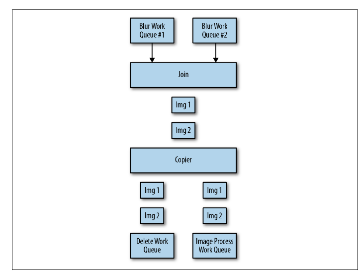
Copier
The first pattern for coordinating work queues is a copier. The job of a copier is to take a single stream of work items and duplicate it out into two or more identical streams. This pattern is useful when there are multiple different pieces of work to be done on the same work item. An example of this might be rendering a video. When rendering a video, there are a variety of different formats that are useful depending on where the video is intended to be shown. There might be a 4-KB high-resolution format for playing off of a hard drive, a 1080-pixel rendering for digital streaming, a low-resolution format for streaming to mobile users on slow networks, and an animated GIF thumbnail for displaying in a movie-picking user interface. All of these work items can be modeled as separate work queues for each render, but the input to each work item is identical.
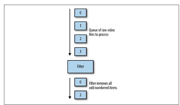
Filter
The second pattern for event-driven batch processing is a filter. The role of a filter is to reduce a stream of work items to a smaller stream of work items by filtering out work items that don’t meet particular criteria. As an example of this, consider setting up a batch workflow that handles new users signing up for a service. Some set of those users will have ticked the checkbox that indicates that they wish to be contacted via email for promotions and other information. In such a workflow, you can filter the set of newly signed-up users to only be those who have explicitly opted into being contacted. Ideally you would compose a filter work queue source as an ambassador that wraps up an existing work queue source. The original source container provides the complete list of items to be worked on, and the filter container then adjusts that list based on the filter criteria and only returns those filtered results to the work queue infrastructure.
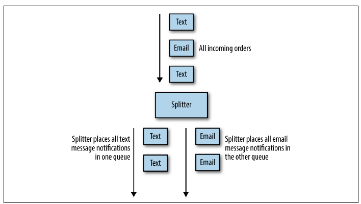
Splitter
Sometimes you don’t want to just filter things out by dropping them on the floor, but rather you have two different kinds of input present in your set of work items and you want to divide them into two separate work queues without dropping any of them. For this task, you want to use a splitter. The role of a splitter is to evaluate some criteria—just like a filter—but instead of eliminating input, the splitter sends different inputs to different queues based on that criteria. An example of an application of the splitter pattern is processing online orders where people can receive shipping notifications either by email or text message. Given a work queue of items that have been shipped, the splitter divides it into two different queues: one that is responsible for sending emails and another devoted to sending text messages. A splitter can also be a copier if it sends the same output to multiple queues, such as when a user selects both text messages and email notifications in the previous example. It is interesting to note that a splitter can actually also be implemented by a copier and two different filters. But the splitter pattern is a more compact representation that captures the job of the splitter more succinctly.
Sharder
A slightly more generic form of splitter is a sharder. Much like the sharded server that we saw in earlier chapters, the role of a sharder in a workflow is to divide up a single queue into an evenly divided collection of work items based upon some sort of sharding function. There are several different reasons why you might consider sharding your workflow. One of the first is for reliability. If you shard your work queue, then the failure of a single workflow due to a bad update, infrastructure failure, or other problem only affects a fraction of your service. For example, imagine that you push a bad update to your worker container, which causes your workers to crash and your queue to stop processing work items. If you only have a single work queue that is processing items, then you will have a complete outage for your service with all users affected. If, instead, you have sharded your work queue into four different shards, you have the opportunity to do a staged rollout of your new worker container. Assuming you catch the failure in the first phase of the staged rollout, sharding your queue into four different shards means that only one quarter of your users would be affected.
An additional reason to shard your work queue is to more evenly distribute work across different resources. If you don’t really care which region or datacenter is used to process a particular set of work items, you can use a sharder to evenly spread work across multiple datacenters to even out utilization of all datacenters/regions. As with updates, spreading your work queue across multiple failure regions also has the bene‐fit of providing reliability against datacenter or region failures.
When the number of healthy shards is reduced due to failures, the sharding algorithm dynamically adjusts to send work to the remaining healthy work queues, even if only a single queue remains.
The last pattern for event-driven or workflow batch systems is a merger. A merger is the opposite of a copier; the job of a merger is to take two different work queues and turn them into a single work queue. Suppose, for example, that you have a large number of different source repositories all adding new commits at the same time. You want to take each of these commits and perform a build-and-test for it. It is not scalable to create a separate build infrastructure for each source repository. We can model each of the different source repositories as a separate work queue source that provides a set of commits. We can transform all of these different work queue inputs into a single merged set of inputs using a merger adapter. This merged stream of commits is then the single source to the build system that performs the actual build. The merger is another great example of the adapter pattern, though in this case, the adapter is actually adapting multiple running source containers into a single merged source.
Building an Event-Driven Flow for New User Sign-Up
A concrete example of a workflow helps show how these patterns can be put together to form a complete operating system. The problem this example will consider is a new-user signup flow. Imagine that our user acquisition funnel has two stages. The first is user verification. After a new user signs up, the user then has to receive an email notification to validate their email. Once the user validates their email, they are sent a confirmation email. Then they are optionally registered for email, text message, both, or neither for notifications. The first step in the event-driven workflow is the generation of the verification email. To achieve this reliably, we will use the shard pattern to shard users across multiple different geographic failure zones. This ensures that we will continue to process new user signups, even in the presence of partial failures. Each work queue shard sends a verification email to the end user. At this point, this substage of the workflow is complete.
Coordinated Batch Processing
Duplicating and producing multiple different outputs is often an important part of batch processing, but sometimes it is equally important to pull multiple outputs back together in order to generate some sort of aggregate output.
Probably the most canonical example of this aggregation is the reduce part of the MapReduce pattern. It’s easy to see that the map step is an example of sharding a work queue, and the reduce step is an example of coordinated processing that eventually reduces a large number of outputs down to a single aggregate response. However, there are a number of different aggregate patterns for batch processing, and this chapter discusses a number of them in addition to real-world applications.
Join (or Barrier Synchronization)
We saw patterns for breaking up work and distributing it in parallel on multiple nodes. In particular, we saw how a sharded work queue could distribute work in parallel to a number of different work queue shards. However, sometimes when processing a workflow, it is necessary to have the complete set of work available to you before you move on to the next stage of the workflow. One option for doing this was shown in the previous chapter, which was to merge multiple queues together. However, merge simply blends the output of two work queues into a single work queue for additional processing. While the merge pattern is sufficient in some cases, it does not ensure that a complete dataset is present prior to the beginning of processing. This means that there can be no guarantees about the completeness of the processing being performed, as well as no opportunity to compute aggregate statistics for all of the elements that have been processed. Instead, we need a stronger, coordinated primitive for batch data processing, and that primitive is the join pattern. Join is similar to joining a thread. The basic idea is that all of the work is happening in parallel, but work items aren’t released out of the join until all of the work items that are processed in parallel are completed. This is also generally known as barrier synchronization in concurrent programming.
Coordination through join ensures that no data is missing before some sort of aggregation phase is performed (e.g., finding the sum of some value in a set). The value of the join is that it ensures that all of the data in the set is present. The downside of the join pattern is that it requires that all data be processed by a previous stage before subsequent computation can begin. This reduces the parallelism that is possible in the batch workflow, and thus increases the overall latency of running the workflow.
Reduce
If sharding a work queue is an example of the map phase of the canonical map/reduce algorithm, then what remains is the reduce phase. Reduce is an example of a coordinated batch processing pattern because it can happen regardless of how the input is split up, and it is used similar to join; that is, to group together the parallel output of a number of different batch operations on different pieces of data. However, in contrast to the join pattern described previously, the goal of reduce is not to wait until all data has been processed, but rather to optimistically merge together all of the parallel data items into a single comprehensive representation of the full set.
With the reduce pattern, each step in the reduce merges several different outputs into a single output. This stage is called “reduce” because it reduces the total number of outputs. Additionally, it reduces the data from a complete data item to simply the representative data necessary for producing the answer to a specific batch computation. Because the reduce phase operates on a range of input, and produces a similar output, the reduce phase can be repeated as many or as few times as necessary in order to successfully reduce the output down to a single output for the entire data set. This is a fortunate contrast to the join pattern, because unlike join, it means that reduce can be started in parallel while there is still processing going on as part of the map/shard phase. Of course, in order to produce a complete output, all of the data must be processed eventually, but the ability to begin early means that the batch computation executes more quickly overall.
To understand how the reduce pattern works, consider the task of counting the number of instances of a particular word in a book. We can first use sharding to divide up the work of counting words into a number of different work queues. As an example, we could create 10 different sharded work queues with 10 different people responsible for counting words in each queue. We can shard the book among these 10 work queues by looking at the page number. All pages that end in the number 1 will go to the first queue, all pages that end in the number 2 will go to the second, and so forth. Once all of the people have finished processing their pages, they write down their results on a piece of paper. For example, they might write:
a: 50
the: 17
cat: 2
airplane: 1
...
This can be output to the reduce phase. Remember that the reduce pattern reduces by
combining two or more outputs into a single output.
Given a second output:
a: 30
the: 25
dog: 4
airplane: 2
...
The reduction proceeds by summing up all of the counts for the various words, in
this example producing:
a: 80
the 42
dog: 4
cat: 2
airplane: 3
...
It’s clear to see that this reduction phase can be repeated on the output of previous reduce phases until there is only a single reduced output left. This is valuable since this means that reductions can be performed in parallel.
Sum
A similar but slightly different form of reduction is the summation of a collection of different values. This is like counting, but rather than simply counting one for every value, you actually add together a value that is present in the original output data. Suppose, for example, you want to sum the total population of the United States. Assume that you will do this by measuring the population in every town and then summing them all together. A first step might be to shard the work into work queues of towns, sharded by state. This is a great first sharding, but it’s clear that even when distributed in parallel, it would take a single person a long time to count the number of people in every town. Consequently, we perform a second sharding to another set of work queues, this time by county. At this point, we have parallelized first to the level of states, then to the level of counties, and then each work queue in each county produces a stream of outputs of (town, population) tuples. Now that we are producing output, the reduce pattern can kick in. In this case, the reduce doesn’t even really need to be aware of the two-level sharding that we performed. It is sufficient for the reduce to simply grab two or more output items, such as (Seattle, 4,000,000) and (Northampton, 25,000), and sum them together to produce a new output (Seattle-Northampton, 4,025,000). It’s clear to see that, like counting, this reduction can be performed an arbitrary number of times with the same code running at each interval, and at the end, there will only be a single output containing the complete population of the United States. Importantly, again, nearly all of the computation required is happening in parallel.
Histogram
As a final example of the reduce pattern, consider that while we are counting the population of the United States via parallel sharding/mapping and reducing, we also want to build a model of the average American family. To do this, we want to develop a histogram of family size; that is, a model that estimates the total number of families with zero to 10 children. We will perform our multi-level sharding exactly as before (indeed, we can likely use the same workers).
However, this time, the output of the data collection phase is a histogram per town.
0: 15%
1: 25%
2: 50%
3: 10%
4: 5%
From the previous examples, we can see that if we apply the reduce pattern, we should be able to combine all of these histograms to develop a comprehensive picture of the United States. At first blush, it may seem quite difficult to understand how to merge these histograms, but when combined with the population data from the summation example, we can see that if we multiply each histogram by its relative population, then we can obtain the total population for each item being merged. If we then divide this new total by the sum of the merged populations, it is clear that we can merge and update multiple different histograms into a single output. Given this, we can apply the reduce pattern as many times as necessary until a single output is produced.
To see how coordinated batch processing can be used to accomplish a larger batch task, consider the job of tagging and processing a set of images. Let us assume that we have a large collection of images of highways at rush hour, and we want to count both the numbers of cars, trucks, and motorcycles, as well as distribution of the colors of each of the cars. Let us also suppose that there is a preliminary step to blur the license plates of all of the cars to preserve anonymity. The images are delivered to us as a series of HTTPS URLs where each URL points to a raw image. The first stage in the pipeline is to find and blur the license plates. To simplify each task in the work queue, we will have one worker that detects a license plate, and a second worker that blurs that location in the image. We will combine these two different worker containers into a single container group using the multiworker pattern described in the previous chapter. This separation of concerns may seem unnecessary, but it is useful given that the workers for blurring images can be reused to blur other outputs (e.g., people’s faces). Additionally, to ensure reliability and to maximize parallel processing, we will shard the images across multiple worker queues.
Once each image has been successfully blurred, we will upload it to a different location, and we will then delete the originals. However, we don’t want to delete the original until all of the images have been successfully blurred in case there is some sort of catastrophic failure and we need to rerun this entire pipeline. Thus, to wait for all of the blurring to complete, we use the join pattern to merge the output of all of the sharded blurring work queues into a single queue that will only release its items after all of the shards have completed the work. Now we are ready to delete the original images as well as begin work on car model and color detection. Again, we want to maximize the throughput of this pipeline, so we will use the copier pattern from the previous chapter to duplicate the work queue items to two different queues:
- A work queue that deletes the original images.
- A work queue that identifies the type of vehicle (car, truck, motorcycle) and the color of the vehicle.
Finally we need to design the queue that identifies vehicles and colors and aggregates these statistics into a final count. To do this, we first again apply the shard pattern to distribute the work out to a number of queues. Each of these queues has two different workers: one that identifies the location and type of each vehicle and one that identifies the color of a region. We will again join these together using the multi-worker pattern described in the previous chapter. As before, the separation of code into different containers enables us to reuse the color detection container for multiple tasks beyond identifying the color of the cars.
This data represents the information found in a single image. To aggregate all of this data together, we will use the reduce pattern described previously and made famous by MapReduce to sum everything together just as we did in the count example above. At the end, this reduce pipeline stage produces the final count of images and colors found in the complete set of images.